BESS Degradation Model
This document explains how battery degradation is calculated in the BESS sizing and simulation code.
Scope of the Degradation Model
The degradation model estimates the loss of usable energy capacity over time. Power capability degradation is explicitly modeled and represented as a reduction in available energy capacity (MWh).
Two degradation mechanisms are modeled:
- Calendar aging
- Cycle aging
Both mechanisms are assumed to be additive and independent.
State Variables
At any simulation step t , the battery state is defined as:
Nominal (nameplate) energy capacity:
Remaining usable energy capacity:
State of Health (SoH):
Battery degradation reduces Et monotonically over time.
Degradation Flow Overview
At each simulation step, degradation is computed using the following sequence:
- Elapsed calendar time is evaluated
- Energy throughput from charging and discharging is accumulated
- Energy throughput is converted to equivalent full cycles
- Calendar aging increment is calculated
- Cycle aging increment is calculated
- Remaining usable capacity is updated
Calendar Aging Model
Calendar aging represents capacity loss that occurs independently of cycling, driven by time-dependent electrochemical processes.
A linear annual degradation model is applied:
Where:
- r_cal is the calendar degradation rate {fraction per year}
- (delta_t) is the elapsed time in years for the simulation step
Typical parameter range:
Calendar degradation accumulates continuously over the full simulation horizon.
Cycle Aging Model
Cycle aging represents degradation caused by energy throughput during charging and discharging.
Energy Throughput
For each time step, total energy throughput is computed as:
Cumulative throughput over time:
Equivalent Full Cycles (EFC)
Rather than counting discrete cycles, degradation is based on equivalent full cycles (EFC):
This formulation correctly accounts for partial cycling and varying depth of discharge.
Incremental EFC for a time step:
Cycle Degradation Calculation
Cycle-related capacity loss is calculated as:
Where:
- r_cycle is degradation per equivalent full cycle {fraction per year}
Typical parameter range:
These values correspond to approximately 2,000–5,000 full cycles to 80% SoH, consistent with grid-scale lithium-ion warranties.
Total Degradation Update
Total degradation per time step is computed as the sum of calendar and cycle contributions:
Remaining usable energy capacity is updated as:
Where E_min is a lower bound on usable capacity to prevent non-physical negative values.
Model Assumptions and Simplifications
The following modeling assumptions are intentionally applied:
- Battery temperature is not explicitly modeled
- C-rate–dependent degradation effects are not differentiated
- Depth-of-discharge dependence is approximated through EFCs
- Power capability degradation is not modeled separately
- Degradation is path-independent and memoryless
These assumptions are appropriate for system-level planning, sizing, and revenue studies, but not for electrochemical design or warranty validation.
Literature and Reference Basis
The degradation structure and parameter ranges are aligned with established literature and standards, including:
- Schmalstieg et al., A holistic aging model for Li(NiMnCo)O₂ based 18650 lithium-ion batteries, Journal of Power Sources, 2014
- Keil & Jossen, Calendar aging of lithium-ion batteries, Journal of The Electrochemical Society, 2017
- EPRI, Battery Energy Storage Overview, 2020
- NREL, Battery Lifetime Analysis and Degradation Modeling, 2019
- IEC 62933-2-1, Electrical Energy Storage Systems – Unit Parameters and Testing
Where explicit numerical values are not defined, mid-range industry values commonly used in grid-scale feasibility studies are applied.
Summary
The degradation model combines calendar aging and cycle aging using a transparent, throughput-based formulation.
It balances physical realism with computational simplicity, making it suitable for energy system modeling where traceability and clarity are more important than electrochemical detail.
Example: BESS Degradation
Asset Definition
Battery Energy Storage System (BESS):
- Power rating: 10 MW
- Energy capacity: 20 MWh
- Nominal duration: 2 hours
- Cycling intensity: 1.5 cycles per day
- Simulation resolution: annual
- Degradation model: linear EFC-based (conservative)
Initial state at beginning of life (BOL):
- Nominal energy capacity:
- Nominal power capacity:
- Initial State of Health:
Degradation Model Configuration
The project uses the following default degradation parameters:
Cycle degradation
- Linear EFC model enabled.
- Fade per equivalent full cycle:
- Default depth-of-discharge factor:
Important:
The model does not assume 80% DoD by default.
Unless a degradation curve is provided, 50% DoD is default.
Depending on the markets selected or trading strategy selected, the model uses the following assumed Depth of Discharge (DoD) (as a percentage):
- If the asset participates in FCR + aFRR + mFRR + Day-ahead + Intraday, we assume 50% DoD.
- If the asset participates in FCR + aFRR + mFRR + Day-ahead, but not Intraday, we assume 40% DoD.
- If the asset participates in Day-ahead only (no Intraday and no balancing services like FCR/aFRR/mFRR), we assume 60% DoD.
- If the asset participates in Day-ahead + Intraday only (no balancing services like FCR/aFRR/mFRR), we assume 60% DoD.
- In all other cases, we assume 60% DoD.
We assume a DoD for a quick analysis although the actual DoD could vary year over year.
Calendar degradation
- Annual calendar fade:
End-of-life
- Minimum State of Health:
Step 1: Cycles per Year
From the operational assumption:
This value is passed directly into the degradation model.
Step 2: Equivalent Full Cycles per Year (Model Logic)
The model computes effective EFCs as:
Step 3: Annual Cycle-Related Degradation
Cycle degradation is computed as a fractional SoH loss:
That is:
Step 4: Annual Calendar Degradation
Calendar degradation is applied linearly:
Step 5: Total Annual SoH Degradation
Step 6: SoH and Energy Capacity Over Time
State of Health after ( n ) years:
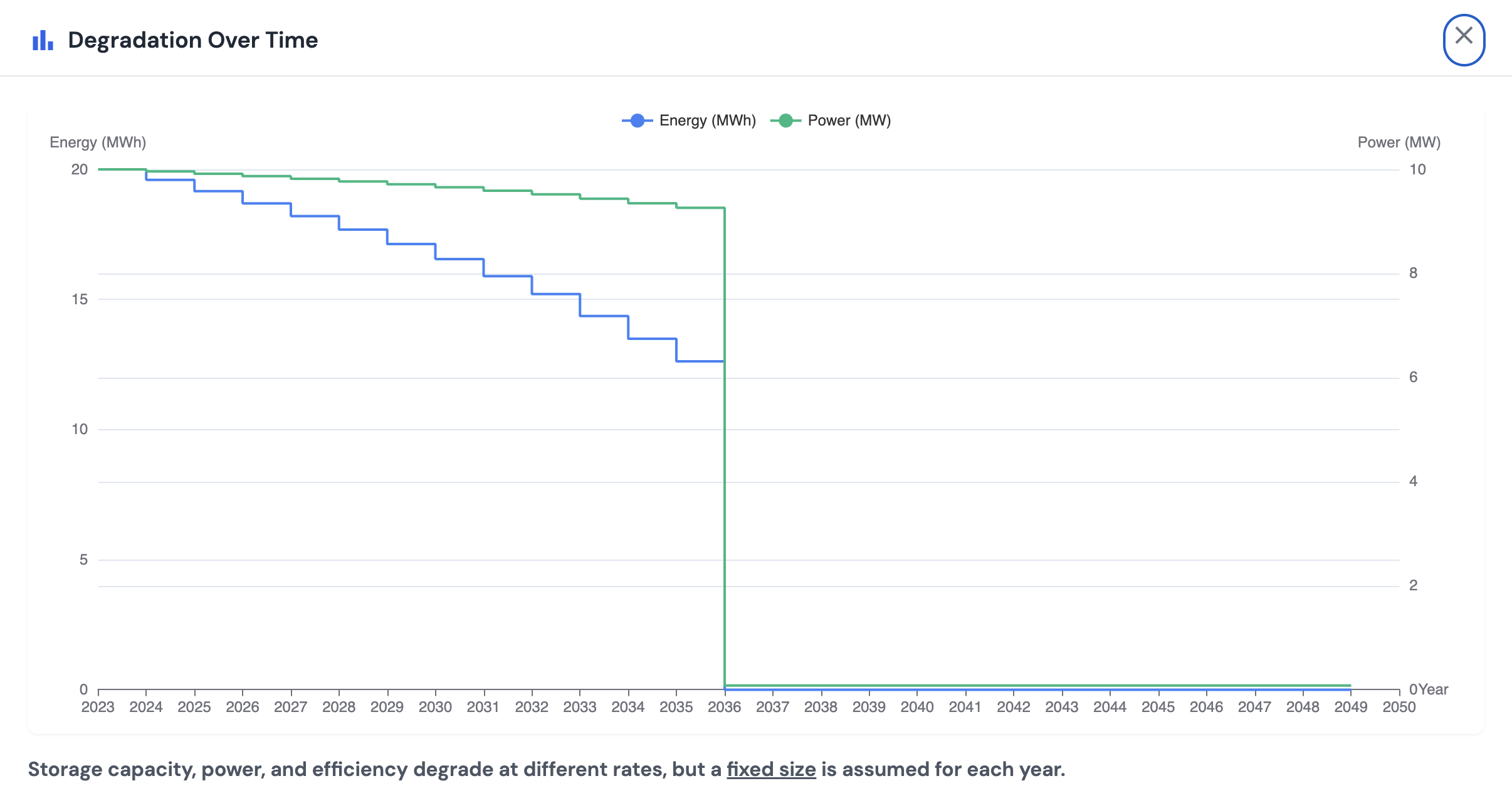
Example: Year 8 (≈ 2031 in chart)
Remaining energy capacity:
This aligns with the gradual stair-step decline in the energy curve.
Step 7: Power Degradation (Model Logic)
Power does not degrade one-to-one with energy.
The model applies a slower power fade using:
Where:
At ~80% SoH:
- Energy ≈ 16–17 MWh
- Power ≈ 9.5–9.6 MW
This matches the tooltip values in the degradation chart.
Interpretation
For a 10 MW / 20 MWh BESS operating at 1.5 cycles per day, the model produces:
- Effective EFCs: ~274 per year
- Annual SoH degradation: ~1.6%
- Gradual energy decline with slower power derating
- End-of-life triggered once SoH reaches 60%
All values shown in the degradation chart are a direct consequence of these calculations.
- Scope of the Degradation Model
- State Variables
- Degradation Flow Overview
- Calendar Aging Model
- Cycle Aging Model
- Total Degradation Update
- Model Assumptions and Simplifications
- Literature and Reference Basis
- Summary
- Asset Definition
- Degradation Model Configuration
- Step 1: Cycles per Year
- Step 2: Equivalent Full Cycles per Year (Model Logic)
- Step 3: Annual Cycle-Related Degradation
- Step 4: Annual Calendar Degradation
- Step 5: Total Annual SoH Degradation
- Step 6: SoH and Energy Capacity Over Time
- Step 7: Power Degradation (Model Logic)
- Interpretation